

When you're working with financial risk data, time matters. Past behavior often hints at future patterns, and that's exactly where recurrent neural networks shine. Unlike traditional neural networks that treat each data point independently, RNNs remember what came before — they're designed for sequences.
Think about credit card transactions or loan default indicators. They're not random events. They're connected in time. A customer's spending patterns last month influence what they might do this month. RNNs capture these temporal dependencies, making them powerful for risk assessment. We'll walk through how to build one from scratch, what makes them tick, and how to avoid the common pitfalls that trip up most practitioners.
Understanding RNN Architecture
RNNs work differently than standard neural networks. They have a hidden state — basically memory — that carries information forward through each timestep. When processing a sequence, the network doesn't just look at the current input. It also considers what happened in previous steps.
The architecture is deceptively simple. At each timestep t, you've got three things: the input data at that step, the hidden state from the previous step, and the output you're predicting. The hidden state gets updated based on both the new input and the old state. It's like keeping notes as you read a book — each chapter adds to what you already know.
There's a catch though. Vanilla RNNs struggle with long sequences. Information from early timesteps gets diluted as it passes through many layers. That's where LSTM (Long Short-Term Memory) cells come in. They've got gates that decide what to remember and what to forget, making them much better at handling longer time horizons — which matters when you're tracking risk over months or years.
Key Architectural Components
- Input layer: Processes timestep data
- Hidden state: Carries temporal memory forward
- LSTM cells: Manage what to remember and forget
- Output layer: Produces risk predictions
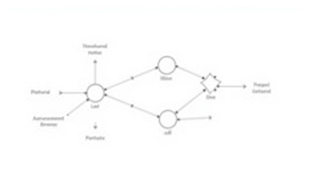
"The power of RNNs lies in their ability to capture dependencies across time. In risk assessment, that temporal context is often the difference between catching emerging problems and missing them entirely."

Building Your First RNN Model
Let's get practical. You'll need historical data organized chronologically — that's non-negotiable. For risk data, you might have 24 months of transaction records, credit scores, or payment histories. The model learns patterns from the first 18 months and gets tested on the remaining 6.
The setup is straightforward. You're building a sequence-to-prediction model. Feed in 30 days of historical data, get out a risk score for day 31. Normalize your inputs — this matters more than people realize. Financial data has huge ranges. Normalizing prevents large values from dominating the learning process and helps the network converge faster.
Your first layer is usually LSTM with 64-128 units. That's enough to capture meaningful temporal patterns without overfitting on smaller datasets. Add dropout between layers — 20-30% is typical. It's insurance against memorizing your training data instead of learning generalizable patterns.
The output layer depends on your task. Binary classification (risky or not)? Use a single neuron with sigmoid activation. Multi-class risk levels (low, medium, high)? Use softmax with three output neurons. Training typically takes 50-100 epochs. You'll know it's working when validation loss stops improving.
Handling Sequence Data Properly
The biggest mistake we see? Treating time series data like regular tabular data. You can't shuffle your sequences randomly — that breaks the temporal structure. If day 5 depends on days 1-4, you need to keep that order intact.
There's also the question of sequence length. Do you look back 7 days? 30 days? 90 days? Longer sequences capture more history but become computationally expensive and harder to train. We typically recommend starting with 30 days for monthly risk assessment and adjusting based on your specific patterns. You'll notice that different risk factors have different temporal horizons. Late payments might show up in weeks, while credit utilization trends take months.
Handling missing data requires care. Don't just fill gaps with zeros — that creates artificial patterns. Instead, use forward-fill (carry the last known value) or interpolation. Better yet, structure your data collection so gaps don't happen in the first place.
Sequence Length
Start with 30 days and adjust based on your validation performance and computational constraints.
Data Normalization
Use StandardScaler on your features. This prevents large values from drowning out subtle patterns.
Train-Test Split
Always use time-based splits. Never randomly shuffle temporal data — it's cheating and won't work in production.


Evaluating Model Performance
Don't just watch accuracy improve. That's misleading with imbalanced datasets — if 95% of your data is "low risk," a model that always predicts low risk gets 95% accuracy but is useless.
Use precision, recall, and F1-score. Precision tells you how many predicted risks are actually risky. Recall tells you how many actual risks you caught. For financial institutions, missing a risky case is usually worse than a false alarm, so you might prioritize recall. The trade-off depends on your business costs.
The confusion matrix is your friend. Look at it every time. See where your model makes mistakes. Are you missing certain types of risk? Misclassifying specific customer segments? This tells you where to focus your data collection or feature engineering efforts.
Don't forget about temporal validation. Test your model on the most recent data it's never seen. Real-world deployment means the model encounters new temporal patterns constantly. If your validation set is old data, you're not seeing how it'll perform on fresh sequences.
Putting It All Together
Building RNNs for time series risk data isn't magic. It's methodical engineering. You've got a solid foundation now — understanding the architecture, preparing sequences properly, building a functional model, and evaluating performance honestly. The next step is experimentation. Take these principles and adapt them to your specific risk domain.
Start simple. A 2-layer LSTM model with standard hyperparameters often outperforms complex architectures that are harder to debug. Monitor your training carefully. Watch for overfitting — if validation loss starts climbing while training loss drops, you're memorizing instead of learning. Adjust dropout, reduce model size, or get more data.
The best part about RNNs? They're interpretable enough to explain to stakeholders, yet powerful enough to catch patterns humans miss. You're building something that actually works in production.
Educational Note
Individual learning outcomes vary from person to person. This guide provides foundational concepts and practical approaches to implementing RNNs for time series analysis. Your specific implementation will depend on your data characteristics, risk domain, and business requirements. Always validate models thoroughly before deploying to production systems.